Part-of-speech tagging (including an example of machine learning)L'étiquetage morphosyntaxique (y compris un exemple d'apprentissage automatique)
PrintedImprimé le·aylart.github.io/learn·
CC BY-NC 4.0
Written in English. The French version was automatically generated
and I have not revised it.
Rédigé en anglais. La version française a été
générée automatiquement et je ne l'ai pas révisée.
Word classes and part-of-speech tagsetsClasses de mots et jeux d'étiquettes morphosyntaxiques
A label for every word
In the sentence Mary loves reading books, you can say of every word
what kind of word it is: a proper noun, a verb, another verb, a noun. Part-of-speech tagging does this automatically for every word of a
text, and the result is written with a tag after each word:
Mary/PROPN loves/VERB reading/VERB books/NOUN.
The classes themselves are older than computers. Grammars have sorted words
into nouns, verbs, adjectives and the rest for two millennia, and the
classes are defined by how a word behaves with its neighbours and by the
endings it takes, not by what it means: a noun is a word that can follow a
determiner and take a plural, whatever it refers to (Jurafsky & Martin,
2026).
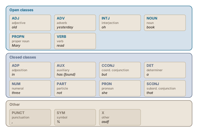
Figure 1. The 17 part-of-speech tags of Universal Dependencies (de Marneffe et al., 2021), with an English example for each.
Classes come in two kinds. Nouns, verbs, adjectives and
adverbs are open classes: new members appear all the time, as selfie
and to google did. Determiners, pronouns, prepositions and conjunctions
are closed classes: a few dozen words each, rarely added to, very frequent,
and doing the structural work of a sentence (Jurafsky & Martin, 2026).
Figure 1figure 1 shows
the seventeen classes of the tagset that Universal Dependencies, a large
collection of annotated corpora, uses for more than a hundred languages (de Marneffe et
al., 2021).
Tagsets differ
Those seventeen tags are one choice among many. A tagset is a decision about
how finely to cut the classes, and different projects have cut them very
differently.
The table below sets some of them side by side, from the seventeen
universal tags to sets that fold number, tense, case or gender into the
tag.The French and Dutch counts were checked on 6 October 2026 at
their sources: TreeTagger’s French tagset,
the label list of a CamemBERT tagger
trained on the French Treebank, and the documentation of the Spoken Dutch
Corpus.
Tagset
Language
Tags
What the extra tags record
Universal Dependencies
more than a hundred languages
17
n.a.; number, tense and gender are expressed as separate features per word
Penn Treebank
English
45
Singular against plural nouns, past tense against past participle, and so on
TreeTagger
French
33
Verb tenses and moods, pronoun types
French Treebank (used by a CamemBERT tagger)
French
29
Verb moods, pronoun types
MULTITAG
French
about 1 500
Gender and number, and for verbs mood and tense, folded into the tag (Allauzen & Bonneau-Maynard, 2008)
Spoken Dutch Corpus (CGN)
Dutch
316
Number, gender, case, tense and more, folded into the tag
Tagsets for Czech, Hungarian, Turkish
languages with rich morphology
4 to 10 times an English set
Case, number and gender (Jurafsky & Martin, 2026)
Tagsets of very different sizes, for the same task.
The information does not disappear when the tagset is small; it is encoded
elsewhere. Universal Dependencies keeps its seventeen tags and records
number, tense or gender as separate features attached to the word (de
Marneffe et al., 2021), where a larger tagset folds them into the tag
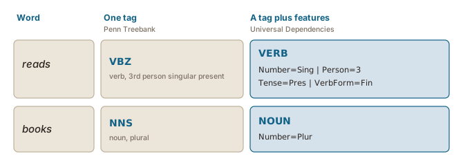
itself. Figure 2figure 2
shows the two conventions on two English words. When you read the output of a
tagger, the first thing to find out is which tagset it used, since ADJ in one and JJ in another may be the same class, and
NN in one may be two classes in another.
Figure 2. The same information in one tag (Penn Treebank) or in a short tag plus features (Universal Dependencies), as mapped by the Universal Dependencies conversion table for the Penn Treebank tags.
Sources
Allauzen, A., & Bonneau-Maynard, H. (2008). Training and Evaluation of POS Taggers on the French MULTITAG Corpus. Proceedings of the Sixth International Conference on Language Resources and Evaluation (LREC'08), Marrakech, 3373–3377. https://aclanthology.org/L08-1368/
de Marneffe, M.-C., Manning, C. D., Nivre, J., & Zeman, D. (2021). Universal Dependencies. Computational Linguistics, 47(2), 255–308. https://doi.org/10.1162/coli_a_00402
Jurafsky, D., & Martin, J. H. (2026). Speech and Language Processing: An Introduction to Natural Language Processing, Computational Linguistics, and Speech Recognition with Language Models. Online draft, 3rd edition. https://web.stanford.edu/~jurafsky/slp3/
Une étiquette pour chaque mot
Dans la phrase Marie adore lire des livres, vous pouvez dire de chaque mot
de quel type de mot il s’agit : un nom propre, un verbe, un autre verbe, un
déterminant, un nom. L’étiquetage morphosyntaxique fait la même chose
automatiquement pour chaque mot d’un texte, et le résultat s’écrit avec une
étiquette après chaque mot :
Marie/PROPN adore/VERB lire/VERB des/DET livres/NOUN.
La tâche prend un texte déjà découpé en
mots (see also the Tokenization (including an example of the rule-based approach) chapter) (voir aussi le chapitre La segmentation en unités lexicales (y compris un exemple d'approche à base de règles)) et donne à
chacun exactement une étiquette (Jurafsky & Martin, 2026). Elle est rarement
le bout d’une chaîne de traitement et presque toujours une étape à
l’intérieur : un concordancier se sert des étiquettes pour vous laisser
chercher tous les noms qui suivent un verbe donné, et un correcteur
grammatical s’en sert, entre autres informations, pour vérifier qu’un verbe
s’accorde avec son sujet.
Classes ouvertes et classes fermées
Les classes elles-mêmes sont plus anciennes que les ordinateurs. Les
grammaires répartissent les mots en noms, verbes, adjectifs et ainsi de suite
depuis deux millénaires, et les classes se définissent par le comportement
d’un mot avec ses voisins et par les terminaisons qu’il prend, non par ce
qu’il veut dire : un nom est un mot qui peut suivre un déterminant et prendre
un pluriel, quoi qu’il désigne (Jurafsky & Martin, 2026).
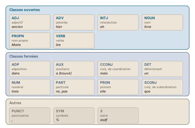
Figure 1. Les 17 étiquettes morphosyntaxiques d'Universal Dependencies (de Marneffe et al., 2021), avec un exemple français pour chacune.
Il y a deux sortes de classes. Les noms, les verbes, les adjectifs et les
adverbes forment des classes ouvertes : de nouveaux membres y entrent sans
cesse, comme courriel et télécharger. Les déterminants, les pronoms, les
prépositions et les conjonctions forment des classes fermées : quelques
dizaines de mots chacune, rarement enrichies, très fréquentes, et qui font le
travail structurel de la phrase (Jurafsky & Martin, 2026).
La Figure 1figure 1 montre les
dix-sept classes du jeu d’étiquettes qu’utilise Universal Dependencies, une
vaste collection de corpus annotés, pour plus de cent langues (de Marneffe et
al., 2021).
Les jeux d’étiquettes diffèrent
Ces dix-sept étiquettes sont un choix parmi d’autres. Un jeu d’étiquettes est
une décision sur la finesse du découpage des classes, et les projets l’ont
tranchée de façons très différentes.
Le tableau ci-dessous en met quelques-uns côte à côte, des dix-sept
étiquettes universelles aux jeux qui intègrent le nombre, le temps, le cas ou
le genre dans l’étiquette.Les chiffres pour le français et le
néerlandais ont été vérifiés le 6 octobre 2026 à leur source : le jeu
d’étiquettes français de TreeTagger,
la liste d’étiquettes d’un étiqueteur CamemBERT
entraîné sur le French Treebank, et la documentation du Spoken Dutch
Corpus.
Jeu d’étiquettes
Langue
Étiquettes
Ce que consignent les étiquettes supplémentaires
Universal Dependencies
plus de cent langues
17
sans objet ; le nombre, le temps et le genre sont exprimés par des traits distincts, mot par mot
Penn Treebank
anglais
45
Nom singulier ou pluriel, passé ou participe passé, etc.
TreeTagger
français
33
Temps et modes du verbe, types de pronoms
French Treebank (utilisé par un étiqueteur CamemBERT)
français
29
Modes du verbe, types de pronoms
MULTITAG
français
environ 1 500
Genre et nombre, et pour les verbes mode et temps, intégrés à l’étiquette (Allauzen & Bonneau-Maynard, 2008)
Spoken Dutch Corpus (CGN)
néerlandais
316
Nombre, genre, cas, temps et plus, intégrés à l’étiquette
Jeux pour le tchèque, le hongrois, le turc
langues à morphologie riche
4 à 10 fois un jeu anglais
Cas, nombre et genre (Jurafsky & Martin, 2026)
Des jeux d'étiquettes de tailles très différentes, pour la même tâche.
L’information ne disparaît pas quand le jeu d’étiquettes est petit : elle est
codée ailleurs. Universal Dependencies garde ses dix-sept étiquettes et
consigne le nombre, le temps ou le genre sous forme de traits distincts
attachés au mot (de Marneffe et al., 2021), là où un jeu plus grand les
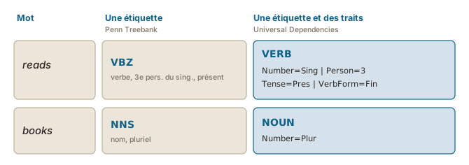
intègre à l’étiquette elle-même. La Figure 2figure 2 montre les deux conventions sur deux mots anglais, puisque le Penn Treebank
est un jeu d’étiquettes pour l’anglais. Quand vous lisez la sortie d’un
étiqueteur, la première chose à vérifier est le jeu d’étiquettes utilisé :
ADJ dans l’un et JJ dans un autre peuvent être la même classe, et NN
dans l’un peut correspondre à deux classes dans un autre.
Figure 2. La même information dans une seule étiquette (Penn Treebank) ou dans une étiquette courte et des traits (Universal Dependencies), selon la table de conversion d'Universal Dependencies pour les étiquettes du Penn Treebank.
Sources
Allauzen, A., & Bonneau-Maynard, H. (2008). Training and Evaluation of POS Taggers on the French MULTITAG Corpus. Proceedings of the Sixth International Conference on Language Resources and Evaluation (LREC'08), Marrakech, 3373–3377. https://aclanthology.org/L08-1368/
de Marneffe, M.-C., Manning, C. D., Nivre, J., & Zeman, D. (2021). Universal Dependencies. Computational Linguistics, 47(2), 255–308. https://doi.org/10.1162/coli_a_00402
Jurafsky, D., & Martin, J. H. (2026). Speech and Language Processing: An Introduction to Natural Language Processing, Computational Linguistics, and Speech Recognition with Language Models. Online draft, 3rd edition. https://web.stanford.edu/~jurafsky/slp3/
Ambiguous word classesL'ambiguïté des classes de mots
One form, several classes
The reason tagging is a task at all is that the form of a word does not
tell you its class. Book is a verb in book that flight and a noun in
hand me that book; fast is an adjective in a fast car and an adverb in
she runs fast. The table below gives four English words with two readings
each.
Word
One reading
The other
book
Hand me that book. (noun)
Book that flight. (verb)
back
She sat in the back. (noun)
Senators back the bill. (verb)
fast
A fast car. (adjective)
She runs fast. (adverb)
that
That book is mine. (determiner)
The book that I read. (relative pronoun)
Four English words that belong to two classes, with a sentence for each reading.
A tagger therefore cannot simply look a word up: it has to assign each
occurrence one of the word’s possible tags. Tagging is a
disambiguation task (Jurafsky & Martin, 2026).
How much of a text is ambiguous
Counted over the word types of a corpus, ambiguity looks like a minor
problem: in two large English corpora, the Wall Street Journal section of
the Penn Treebank (Marcus et al., 1993) and the Brown corpus (Francis &
Kučera, 1979), about 85 % of
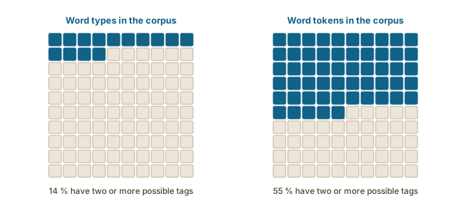
the types have a single possible tag. Counted over the word tokens, it is the
normal case: the
ambiguous types are among the most frequent words of the language, and 55 to
67 % of the tokens in those corpora are ambiguous (Jurafsky & Martin, 2026). Figure 3figure 3
shows the two counts for the Wall Street Journal.
Figure 3. Ambiguity counted over word types and over tokens in the Wall Street Journal section of the Penn Treebank (Jurafsky & Martin, 2026). In the Brown corpus the figures are 15 % and 67 %.
The words with the most readings are short function words and common verbs:
in English that, back, down, put and set; back alone can take six
tags (Jurafsky & Martin, 2026). Word classes are one kind of ambiguity among
several, and frequency goes with the others too. Piantadosi et al. (2012)
found that in English, German and Dutch, more frequent word forms have more
homophones, and that in English more frequent words have more senses, even
with word length taken into account, a link Zipf had already observed. They
read it as efficiency: short, frequent forms are easy to produce and to
process, so a language reuses them for several meanings and leaves the
context to tell them apart.
Where annotators disagree
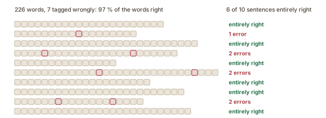
Ambiguity is not only a problem for programs. When people tag a corpus by
hand, following written guidelines, they agree on about 97 % of the tags,
and many of the remaining 3 % are cases where the grammar gives no clean
answer (Manning, 2011). English -ing forms before a noun are the
classic case, and the table below applies one test to three of them: an
adjective takes very, a verb form does not.
Phrase
With very
Reading
a boring lecture
a very boring lecture works
adjective
the falling leaves
the very falling leaves does not
verb form
sparkling lemonade
very sparkling lemonade: doubtful
between the two, for the guidelines to settle
Three -ing forms before a noun, and what the very test says about each.
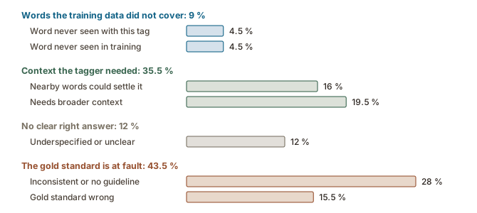
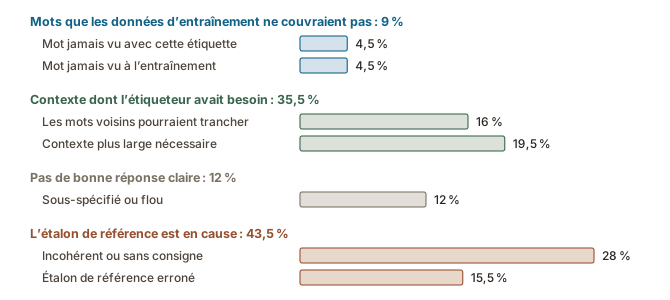
Figure 4. A hundred errors of an English tagger on Wall Street Journal text, in the seven classes of Manning (2011), grouped as he discusses them; an error that fitted two classes counted half in each.
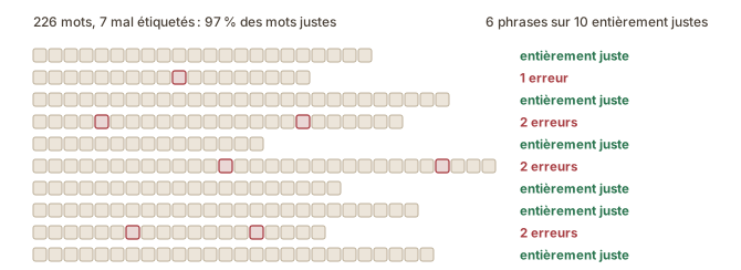
Figure 5. An illustration of what 97 % accuracy means.
Sources
Francis, W. N., & Kučera, H. (1979). Manual of information to accompany a standard corpus of present-day edited American English, for use with digital computers. Department of Linguistics, Brown University, Providence, RI (revised and amplified edition; first published 1964). https://listings.lib.msu.edu/public-corpora/cd421/manuals/brown/INDEX.HTM
Jurafsky, D., & Martin, J. H. (2026). Speech and Language Processing: An Introduction to Natural Language Processing, Computational Linguistics, and Speech Recognition with Language Models. Online draft, 3rd edition. https://web.stanford.edu/~jurafsky/slp3/
Manning, C. D. (2011). Part-of-speech tagging from 97% to 100%: Is it time for some linguistics?. In A. Gelbukh (Ed.), Computational Linguistics and Intelligent Text Processing, CICLing 2011 (Lecture Notes in Computer Science, Vol. 6608, pp. 171–189). Springer. https://doi.org/10.1007/978-3-642-19400-9_14
Marcus, M. P., Santorini, B., & Marcinkiewicz, M. A. (1993). Building a Large Annotated Corpus of English: The Penn Treebank. Computational Linguistics, 19(2), 313–330. https://aclanthology.org/J93-2004/
Si l’étiquetage est une tâche, c’est parce que la forme d’un mot ne dit pas
sa classe. Marche est un verbe dans je marche lentement et un nom dans
une marche en forêt ; fort est un adjectif dans un homme fort et un
adverbe dans il travaille fort. Le tableau ci-dessous donne quatre mots
français à deux lectures.
Mot
Une lecture
L’autre
marche
Je marche lentement. (verbe)
Une marche en forêt. (nom)
livre
Elle me donne un livre. (nom)
Il livre ses pensées. (verbe)
fort
Un homme fort. (adjectif)
Il travaille fort. (adverbe)
que
Le garçon que je vois. (pronom relatif)
Je crois que tu as raison. (conjonction de subordination)
Quatre mots français qui appartiennent à deux classes, avec une phrase pour chaque lecture.
Un étiqueteur ne peut donc pas simplement chercher un mot dans une liste : il
doit attribuer à chaque occurrence l’une des étiquettes possibles du mot.
L’étiquetage est une tâche de désambiguïsation (Jurafsky & Martin, 2026).
Quelle part d’un texte est ambiguë
Comptée sur les types de mots d’un corpus, l’ambiguïté semble un problème
mineur : dans deux grands corpus anglais, la section Wall Street Journal du
Penn Treebank (Marcus et al., 1993) et le corpus Brown (Francis & Kučera,
1979), environ 85 % des
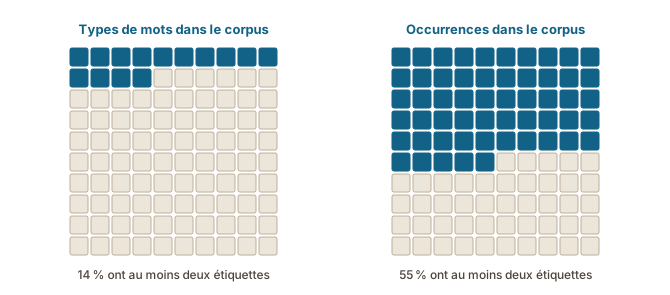
types n’ont qu’une étiquette possible. Comptée sur les occurrences, elle est
la norme : les types ambigus sont parmi les mots les plus fréquents de la
langue, et 55 à 67 % des occurrences de ces corpus sont ambiguës (Jurafsky &
Martin, 2026). La Figure 3figure 3 montre les deux comptes pour le Wall Street Journal.
Figure 3. L'ambiguïté comptée sur les types et sur les occurrences dans la section Wall Street Journal du Penn Treebank (Jurafsky & Martin, 2026). Dans le corpus Brown, les chiffres sont de 15 % et 67 %.
Les mots qui ont le plus de lectures sont de petits mots grammaticaux et des
verbes courants : en anglais that, back, down, put et set ; back
peut à lui seul prendre six étiquettes (Jurafsky & Martin, 2026). Les classes
de mots sont une forme d’ambiguïté parmi d’autres, et la fréquence va de pair
avec les autres aussi. Piantadosi et al. (2012) ont constaté qu’en anglais, en
allemand et en néerlandais, les formes de mots les plus fréquentes ont plus
d’homophones, et qu’en anglais les mots les plus fréquents ont plus de sens,
même à longueur égale, un lien que Zipf avait déjà observé. Ils y voient une
question d’efficacité : les formes courtes et fréquentes sont faciles à
produire et à traiter, si bien qu’une langue les réutilise pour plusieurs sens
et laisse au contexte le soin de les distinguer.
Là où les annotateurs divergent
L’ambiguïté n’est pas un problème réservé aux programmes. Quand des personnes
étiquettent un corpus à la main en suivant des consignes écrites, elles
s’accordent sur environ 97 % des étiquettes, et bien des 3 % restants sont des
cas où la grammaire ne donne pas de réponse nette (Manning, 2011). En
anglais, les formes en -ing devant un nom sont le cas classique, et le
tableau ci-dessous applique un test à trois d’entre elles : un adjectif
accepte very (« très »), une forme verbale non.
Expression
Avec very
Lecture
a boring lecture
a very boring lecture fonctionne
adjectif
the falling leaves
the very falling leaves ne fonctionne pas
forme verbale
sparkling lemonade
very sparkling lemonade : douteux
entre les deux, aux consignes de trancher
Trois formes en -ing devant un nom, et ce qu'en dit le test de very.
Figure 4. Cent erreurs d'un étiqueteur anglais sur des textes du Wall Street Journal, dans les sept classes de Manning (2011), regroupées comme il les discute ; une erreur qui relevait de deux classes comptait pour moitié dans chacune.
Figure 5. Une illustration de ce que signifie une exactitude de 97 %.
Sources
Francis, W. N., & Kučera, H. (1979). Manual of information to accompany a standard corpus of present-day edited American English, for use with digital computers. Department of Linguistics, Brown University, Providence, RI (revised and amplified edition; first published 1964). https://listings.lib.msu.edu/public-corpora/cd421/manuals/brown/INDEX.HTM
Jurafsky, D., & Martin, J. H. (2026). Speech and Language Processing: An Introduction to Natural Language Processing, Computational Linguistics, and Speech Recognition with Language Models. Online draft, 3rd edition. https://web.stanford.edu/~jurafsky/slp3/
Manning, C. D. (2011). Part-of-speech tagging from 97% to 100%: Is it time for some linguistics?. In A. Gelbukh (Ed.), Computational Linguistics and Intelligent Text Processing, CICLing 2011 (Lecture Notes in Computer Science, Vol. 6608, pp. 171–189). Springer. https://doi.org/10.1007/978-3-642-19400-9_14
Marcus, M. P., Santorini, B., & Marcinkiewicz, M. A. (1993). Building a Large Annotated Corpus of English: The Penn Treebank. Computational Linguistics, 19(2), 313–330. https://aclanthology.org/J93-2004/
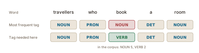
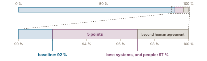
Figure 6. The most frequent tag on a phrase from the small corpus of the worked example. Figure 7. Part-of-speech tagging of English: the share of words tagged correctly by the baseline, and by the best systems and by people, with the top of the scale enlarged (Jurafsky & Martin, 2026).
Looking at the previous word
So the challenge is to get from 92 % as close as possible to 97 %. The errors
that remain with the naive approach, always using a word’s most frequent tag,
mostly come from ambiguous words with more than one possible tag, such as book,
which can be a verb or a noun
(Figure 6figure 6).
To disambiguate such a word, a tagger looks at its context, and a first step
is to look not only at the word that needs a tag, but also at the word before
it. A bigram is a
sequence of two consecutive words, or here of two consecutive tags, and a
bigram tagger adds a second count to the first: how often each tag follows the
tag of the previous word (Jurafsky & Martin, 2026). The bigram is one case of
a general notion, the n-gram, a sequence of n consecutive items: a trigram
tagger, for instance, looks at the tags of the two previous words.
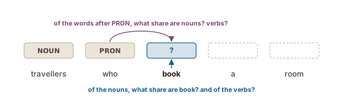
Figure 8. The two questions a bigram tagger asks to tag book in travellers who book a room.
The tagger answers the two questions of
Figure 8figure 8 with
two probabilities, both counted in the tagged corpus, and gives the word the
tag for which the two together score highest.
Reading a probability such as P(book | VERB)
A probability is a share: a number between 0 and 1 that says how often
something happens out of a set of cases. 0 means never, 1 means always, and
0.25 means one time in four, or 25 %.
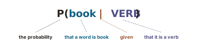
The notation P(A | B) is read “the probability of A, given B”. The bar means
given, and what comes after it says which cases you count in. Figure 9figure 9
reads P(book | VERB) piece by piece, and the table below reads both
probabilities a bigram tagger uses.
Figure 9. Reading P(book | VERB).
Written
Read as
Counted as
P(book | VERB)
the probability that a word is book, given that it is a verb
of all the verbs in the corpus, the share that are book
P(VERB | PRON)
the probability that a tag is VERB, given that the previous tag is PRON
of all the words that follow a pronoun, the share that are verbs
The two probabilities of a bigram tagger, read aloud and counted.
Both probabilities are plain shares, so you can work them out by hand.
A worked example, step by step
The phrase is travellers who book a room, and the counts come from a
small corpus of eight short English sentences, tagged by hand, in which
book occurs seven times in the singular (the plural books is another form), five times as a noun and twice as a verb. Figure 10figure 10
builds up with the four steps below.
Click the drawing, or a line below, to build it up stage by stage.Cliquez sur le dessin, ou sur une ligne ci-dessous, pour le construire étape par étape.
Figure 10. The worked example for book in travellers who book a room, one stage per step.
Step 1: the candidate tags
Figure 11. Stage 1 of the worked example.
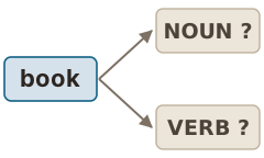
A tagger does not invent a tag: it compares the tags a word can have. The
corpus shows two for book, NOUN and VERB, so the tagger computes one score
for each, and the higher score wins (Figure 11figure 11).
Step 2: the word, given each tag
Figure 12. Stage 2 of the worked example.
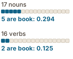
The first question counts, of the words that carry each tag, the share that
are book: among the nouns first, then among the verbs, and not among the
occurrences of book
(Figure 12figure 12).
5 of the 17 nouns are book: 0.294, written P(book | NOUN);
2 of the 16 verbs are book: 0.125, written P(book | VERB).
On this question alone, NOUN is ahead. That is the most frequent tag again,
and it is wrong here: the word on its own cannot tell this book from the
noun.
Step 3: each tag, given the previous tag
Figure 13. Stage 3 of the worked example.
The second question is what usually comes after the previous tag, which is
the information the most frequent tag never used. The word before book is
who, a pronoun, and the corpus has 9 words after a pronoun
(Figure 13figure 13).
none of them is a noun: 0, written P(NOUN | PRON);
4 of them are verbs: 0.444, written P(VERB | PRON).
Step 4: combining the two
Figure 14. Stage 4 of the worked example.
The tagger needs one score per tag that takes both answers into account, so
it multiplies them (Figure 14figure 14). A product is high only when
both numbers are, and a zero in either makes the whole product zero:
NOUN scores 0.294 × 0 = 0, and VERB scores 0.125 × 0.444 = 0.056.
VERB wins. The previous tag has overturned the lead NOUN had on the word
alone, and the tagger labels this book a verb, although book is a noun
more often than not.
A count of zero decided this case, and in a corpus of a hundred words that
happens all the time: a noun can follow a pronoun in English, as in her
book, where Universal Dependencies tags her as a pronoun, but the corpus
contains no example of it. Real taggers correct for this by giving every
count a small minimum, so that a sequence never seen in the corpus is
unlikely rather than impossible (Jurafsky & Martin, 2026).
The method as a rule
For every word of a text, a bigram tagger does the same three things with
counts from a tagged corpus:
it lists the tags the word can have;
for each tag, it multiplies the share of the word among the words that
carry this tag, P(word | tag), by the share of this tag
among the words that follow the previous tag,
P(tag | previous tag);
it keeps the tag with the larger product.
No rule anywhere says that book after who is a verb, and the method never
uses what book means: the counts alone decide.
Jurafsky, D., & Martin, J. H. (2026). Speech and Language Processing: An Introduction to Natural Language Processing, Computational Linguistics, and Speech Recognition with Language Models. Online draft, 3rd edition. https://web.stanford.edu/~jurafsky/slp3/
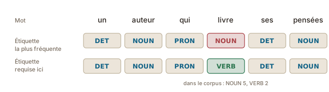
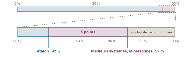
Figure 6. L'étiquette la plus fréquente sur un segment du petit corpus de l'exemple détaillé. Figure 7. Étiquetage morphosyntaxique de l'anglais : la proportion de mots étiquetés correctement par l'étalon, par les meilleurs systèmes et par des personnes, avec le haut de l'échelle agrandi (Jurafsky & Martin, 2026).
Regarder le mot précédent
Le défi est donc de passer de 92 % au plus près de 97 %. Les erreurs qui
restent avec l’approche naïve, toujours prendre l’étiquette la plus fréquente
d’un mot, viennent surtout des mots ambigus qui ont plus d’une étiquette
possible, comme livre, qui peut être un verbe ou un nom
(Figure 6figure 6).
Pour lever l’ambiguïté d’un tel mot, un étiqueteur regarde son contexte, et
une première étape consiste à regarder non seulement le mot à étiqueter, mais
aussi le mot qui le précède. Un bigramme est une suite de deux mots
consécutifs, ou ici de deux étiquettes consécutives, et un étiqueteur
bigramme ajoute un second compte au premier : la fréquence de chaque étiquette
après l’étiquette du mot précédent (Jurafsky & Martin, 2026). Le bigramme est
un cas d’une notion générale, le n-gramme, une suite de n éléments
consécutifs : un étiqueteur trigramme, par exemple, regarde les étiquettes
des deux mots précédents.
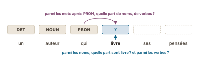
Figure 8. Les deux questions que pose un étiqueteur bigramme pour étiqueter livre dans un auteur qui livre ses pensées.
L’étiqueteur répond aux deux questions de
Figure 8figure 8 par deux
probabilités, toutes deux comptées dans le corpus étiqueté, et donne au mot
l’étiquette pour laquelle les deux ensemble obtiennent le meilleur score.
Lire une probabilité comme P(livre | VERB)
Une probabilité est une proportion : un nombre entre 0 et 1 qui dit combien
de fois quelque chose se produit dans un ensemble de cas. 0 veut dire jamais,
1 toujours, et 0,25 une fois sur quatre, soit 25 %.
La notation P(A | B) se lit « la probabilité de A sachant
B ». La barre veut dire sachant, et ce qui la suit dit parmi quels cas on
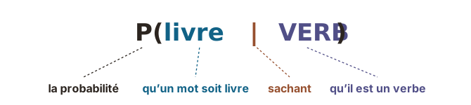
compte. La Figure 9figure 9 lit
P(livre | VERB) morceau par morceau, et le tableau
ci-dessous lit les deux probabilités qu’utilise un étiqueteur bigramme.
Figure 9. Lire P(livre | VERB).
Notation
Se lit
Se compte
P(livre | VERB)
la probabilité qu’un mot soit livre, sachant que c’est un verbe
parmi tous les verbes du corpus, la proportion qui sont livre
P(VERB | PRON)
la probabilité qu’une étiquette soit VERB, sachant que l’étiquette précédente est PRON
parmi tous les mots qui suivent un pronom, la proportion de verbes
Les deux probabilités d'un étiqueteur bigramme, lues à voix haute et comptées.
Les deux probabilités sont de simples proportions, et vous pouvez les
calculer à la main.
Un exemple détaillé, étape par étape
Le segment est un auteur qui livre ses pensées, et les comptes viennent d’un
petit corpus de huit courtes phrases françaises, étiquetées à la main, où
livre apparaît sept fois au singulier (le pluriel livres est une autre forme), cinq fois comme nom et deux fois comme verbe. La Figure 10figure 10 se construit au fil des quatre étapes ci-dessous.
Click the drawing, or a line below, to build it up stage by stage.Cliquez sur le dessin, ou sur une ligne ci-dessous, pour le construire étape par étape.
Figure 10. L'exemple détaillé pour livre dans un auteur qui livre ses pensées, une phase par étape.
Étape 1 : les étiquettes candidates
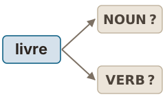
Figure 11. Étape 1 de l'exemple détaillé.
Un étiqueteur n’invente pas d’étiquette : il compare les étiquettes qu’un mot
peut avoir. Le corpus en montre deux pour livre, NOUN et VERB, donc
l’étiqueteur calcule un score pour chacune, et le plus haut l’emporte
(Figure 11figure 11).
Étape 2 : le mot, sachant chaque étiquette
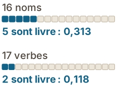
Figure 12. Étape 2 de l'exemple détaillé.
La première question compte, parmi les mots qui portent chaque étiquette, la
part qui sont livre : parmi les noms d’abord, puis parmi les verbes, et non
parmi les occurrences de livre
(Figure 12figure 12).
5 des 16 noms sont livre : 0,313, qui s’écrit P(livre | NOUN) ;
2 des 17 verbes sont livre : 0,118, qui s’écrit P(livre | VERB).
Sur cette seule question, NOUN est en tête. C’est encore l’étiquette la plus
fréquente, et elle est fausse ici : le mot seul ne permet pas de distinguer ce
livre du nom.
Étape 3 : chaque étiquette, sachant l’étiquette précédente
Figure 13. Étape 3 de l'exemple détaillé.
La seconde question porte sur ce qui vient d’habitude après l’étiquette
précédente, l’information que l’étiquette la plus fréquente n’utilisait
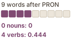
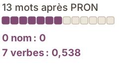
jamais. Le mot avant livre est qui, un pronom, et le corpus compte 13
mots après un pronom
(Figure 13figure 13).
aucun n’est un nom : 0, qui s’écrit P(NOUN | PRON) ;
7 sont des verbes : 0,538, qui s’écrit P(VERB | PRON).
Étape 4 : combiner les deux
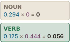
Figure 14. Étape 4 de l'exemple détaillé.
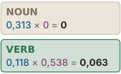
L’étiqueteur a besoin d’un score par étiquette qui tienne compte des deux
réponses, et il les multiplie
(Figure 14figure 14). Un
produit n’est élevé que si les deux nombres le sont, et un zéro dans l’un des
deux annule le produit entier : NOUN obtient 0,313 × 0 = 0,
et VERB 0,118 × 0,538 = 0,063.
VERB l’emporte. L’étiquette précédente a renversé l’avance que NOUN avait sur
le mot seul, et l’étiqueteur étiquette ce livre comme un verbe, alors que
livre est le plus souvent un nom.
Un compte nul a décidé ce cas, et dans un corpus d’une centaine de mots, cela
arrive tout le temps : une séquence absente du corpus devient impossible,
alors qu’elle n’est que rare. Les vrais étiqueteurs corrigent ce problème en
donnant à chaque compte un petit minimum, de sorte qu’une séquence jamais vue
dans le corpus soit improbable plutôt qu’impossible (Jurafsky & Martin, 2026).
La méthode comme règle
Pour chaque mot d’un texte, un étiqueteur bigramme fait les trois mêmes
choses avec des comptes tirés d’un corpus étiqueté :
il fait la liste des étiquettes que le mot peut avoir ;
pour chaque étiquette, il multiplie la part du mot parmi les mots qui
portent cette étiquette, P(mot | étiquette), par la part
de cette étiquette parmi les mots qui suivent l’étiquette précédente,
P(étiquette | étiquette précédente) ;
il garde l’étiquette dont le produit est le plus grand.
Aucune règle ne dit nulle part que livre après qui est un verbe, et la
méthode n’utilise jamais ce que livre veut dire : seuls les comptes
décident.
Jurafsky, D., & Martin, J. H. (2026). Speech and Language Processing: An Introduction to Natural Language Processing, Computational Linguistics, and Speech Recognition with Language Models. Online draft, 3rd edition. https://web.stanford.edu/~jurafsky/slp3/
Practice: tagging watch with probabilitiesExercices : étiqueter montre avec des probabilités
To answer, count in the corpus: all the nouns and all the verbs, those that
are the form watch, and what follows each pronoun and each punctuation
mark. Each line is one sentence, and you count what follows a word inside
its sentence: the final full stop is followed by nothing. The probabilities
are shares, so write them as decimals or as percentages, rounded to two
decimals.
Exercises
ExerciseExercice 1 · the word given the tag, for the nounle mot sachant l'étiquette, pour le nomnot startedà fairesolvedréussikeep tryingà retravailler
The tagger's first question: how typical watch is of nouns. Count all the words tagged NOUN in the corpus, then those that are the form watch. What is P(watch | NOUN)? Round to two decimals.
Première question de l'étiqueteur : à quel point « montre » est typique des noms. Comptez tous les mots étiquetés NOUN dans le corpus, puis ceux qui sont la forme « montre ». Quelle est P(montre | NOUN) ? Arrondissez à deux décimales.
Show the explanationVoir l'explication
The corpus has 21 nouns, of which 2 are watch (an old watch, a watch needs). P(watch | NOUN) = 2 / 21 = 0.10, or 9.52 %.
Le corpus compte 21 noms, dont 2 sont « montre » (« une montre en or », « qu'une montre demande »). P(montre | NOUN) = 2 / 21 = 0,10, soit 9,52 %.
ExerciseExercice 2 · the word given the tag, for the verble mot sachant l'étiquette, pour le verbenot startedà fairesolvedréussikeep tryingà retravailler
The same calculation for verbs: what is P(watch | VERB)? Count all the verbs, then those that are the form watch. Round to two decimals.
Le même calcul pour les verbes : quelle est P(montre | VERB) ? Comptez tous les verbes, puis ceux qui sont la forme « montre ». Arrondissez à deux décimales.
Show the explanationVoir l'explication
The corpus has 13 verbs, of which 3 are watch (the children watch, Visitors watch, Lea and Tom watch). P(watch | VERB) = 3 / 13 = 0.23, or 23.08 %. On the word alone, VERB is ahead: watch is a verb more often than a noun in the corpus.
Le corpus compte 12 verbes, dont 3 sont « montre » (« lui montre », « un guide montre », « Léa montre »). P(montre | VERB) = 3 / 12 = 0,25. « Montrant » est un verbe mais une autre forme : il compte parmi les 12 verbes, pas parmi les « montre ». Sur le mot seul, VERB est en tête : « montre » est plus souvent un verbe qu'un nom dans le corpus.
ExerciseExercice 3 · the tag given the previous tag, for the nounl'étiquette sachant l'étiquette précédente, pour le nomnot startedà fairesolvedréussikeep tryingà retravailler
The second question: what usually follows the previous tag. In she checks her watch, the word before watch is her, which Universal Dependencies tags as a pronoun (PRON), possessive or not. Count all the words that follow a pronoun in the corpus, then those that are nouns. What is P(NOUN | PRON)? Round to two decimals.
Seconde question : ce qui suit d'habitude l'étiquette précédente. Dans « un bracelet de montre », le mot avant « montre » est « de », une préposition (ADP). Comptez tous les mots qui suivent une préposition dans le corpus, puis ceux qui sont des noms. Quelle est P(NOUN | ADP) ? Arrondissez à deux décimales.
Show the explanationVoir l'explication
The corpus has 9 pronouns, and 4 are followed by a noun: her wrist, Her grandfather, their garden and his apprentices. P(NOUN | PRON) = 4 / 9 = 0.44, or 44.44 %. Of the other five, two are followed by punctuation, one by an adverb, one by an auxiliary and one by a verb.
Le corpus compte 10 prépositions, et 4 sont suivies d'un nom : « en or », « avec attention », « d'horlogerie » et « en silence ». P(NOUN | ADP) = 4 / 10 = 0,40. Cinq autres sont suivies d'un déterminant, comme « à le poignet », et la dernière d'un verbe.
ExerciseExercice 4 · the tag given the previous tag, for the verbl'étiquette sachant l'étiquette précédente, pour le verbenot startedà fairesolvedréussikeep tryingà retravailler
The same calculation for verbs: what is P(VERB | PRON)? Round to two decimals.
Le même calcul pour les verbes : quelle est P(VERB | ADP) ? Arrondissez à deux décimales.
Show the explanationVoir l'explication
Only one of the 9 pronouns is followed by a verb: He explains. P(VERB | PRON) = 1 / 9 = 0.11, or 11.11 %. This count covers every verb, whatever its form: here the tagger only looks at the tags.
Une seule des 10 prépositions est suivie d'un verbe : « à croire ». P(VERB | ADP) = 1 / 10 = 0,10. Ce compte porte sur tous les verbes, quelle que soit leur forme : l'étiqueteur ne regarde ici que les étiquettes.
Which tag does the bigram tagger give watch in She checks her watch, and why?
Quelle étiquette l'étiqueteur bigramme donne-t-il à « montre » dans « Elle cherche un bracelet de montre », et pourquoi ?
Show the solutionVoir la solution
The tagger compares two products: for the noun, 0.0952 × 0.444 = 0.042; for the verb, 0.231 × 0.111 = 0.026. The noun wins.
The first answer is the most frequent tag: on the word alone, VERB was ahead, and the tag would be wrong. The previous tag overturns the verb's lead, as in the worked example but the other way round. The third answer gives the right tag for the wrong reason: the tagger only knows that the previous tag is PRON, and nothing about possessives. The fourth forgets that the tagger never looks for the sentence in the corpus: it combines two counts, and both are there.
L'étiqueteur compare deux produits : pour le nom, 0,0952 × 0,40 = 0,038 ; pour le verbe, 0,25 × 0,10 = 0,025. Le nom l'emporte.
La première réponse est l'étiquette la plus fréquente : sur le mot seul, VERB était en tête, et l'étiquette serait fausse. C'est l'étiquette précédente qui renverse l'avance du verbe, comme dans l'exemple détaillé, mais dans l'autre sens. La troisième réponse donne la bonne étiquette pour une mauvaise raison : l'étiqueteur bigramme regarde l'étiquette du mot précédent, ADP pour « de », et non le mot « bracelet ». La quatrième oublie que l'étiqueteur ne cherche jamais la phrase dans le corpus : il combine deux comptes, et tous deux s'y trouvent.
Which tag does the bigram tagger give watch in He waits, watch in hand, and is the tag right?
Quelle étiquette l'étiqueteur bigramme donne-t-il à « montre » dans « Il attend, montre en main », et cette étiquette est-elle juste ?
Show the solutionVoir la solution
The previous word is the comma, tagged PUNCT. In the corpus, four words follow punctuation inside a sentence: one is a verb (, pointing) and none is a noun. The product for NOUN is therefore 0, and the product for VERB is small but positive: 0.231 × 1 / 4 = 0.058. VERB wins, and the tag is wrong: in watch in hand, watch is a noun.
The method works exactly as it should: the corpus has no noun after punctuation, so a zero decides the case. Real taggers give every count a small minimum for this reason. The first answer credits the tagger with a look at the next word, which is not part of its two counts, and the second describes the most frequent tag, which the bigram tagger does not use on its own.
Le mot précédent est la virgule, étiquetée PUNCT. Dans le corpus, six mots suivent une ponctuation à l'intérieur d'une phrase : un seul est un verbe (« , montrant ») et aucun n'est un nom. Le produit pour NOUN vaut donc 0, et celui pour VERB est petit mais positif : 0,25 × 1 / 6 = 0,042. VERB l'emporte, et l'étiquette est fausse : dans « montre en main », « montre » est un nom.
La méthode fonctionne exactement comme prévu : le corpus ne contient aucun nom après une ponctuation, si bien qu'un zéro tranche le cas. C'est pour cette raison que les vrais étiqueteurs donnent à chaque compte un petit minimum. La première réponse prête à l'étiqueteur un regard sur le mot suivant, qui ne fait pas partie de ses deux comptes, et la deuxième décrit l'étiquette la plus fréquente, que l'étiqueteur bigramme n'utilise pas seule.
Pour répondre, comptez dans le corpus : tous les noms et tous les verbes,
ceux qui sont la forme montre, et ce qui suit chaque préposition et chaque
ponctuation. Chaque ligne est une phrase, et on compte ce qui suit un mot à
l’intérieur de sa phrase : le point final n’est suivi de rien. Les
probabilités sont des proportions : écrivez-les en décimales ou en
pourcentages, arrondies à deux décimales.
Exercices
ExerciseExercice 1 · the word given the tag, for the nounle mot sachant l'étiquette, pour le nomnot startedà fairesolvedréussikeep tryingà retravailler
The tagger's first question: how typical watch is of nouns. Count all the words tagged NOUN in the corpus, then those that are the form watch. What is P(watch | NOUN)? Round to two decimals.
Première question de l'étiqueteur : à quel point « montre » est typique des noms. Comptez tous les mots étiquetés NOUN dans le corpus, puis ceux qui sont la forme « montre ». Quelle est P(montre | NOUN) ? Arrondissez à deux décimales.
Show the explanationVoir l'explication
The corpus has 21 nouns, of which 2 are watch (an old watch, a watch needs). P(watch | NOUN) = 2 / 21 = 0.10, or 9.52 %.
Le corpus compte 21 noms, dont 2 sont « montre » (« une montre en or », « qu'une montre demande »). P(montre | NOUN) = 2 / 21 = 0,10, soit 9,52 %.
ExerciseExercice 2 · the word given the tag, for the verble mot sachant l'étiquette, pour le verbenot startedà fairesolvedréussikeep tryingà retravailler
The same calculation for verbs: what is P(watch | VERB)? Count all the verbs, then those that are the form watch. Round to two decimals.
Le même calcul pour les verbes : quelle est P(montre | VERB) ? Comptez tous les verbes, puis ceux qui sont la forme « montre ». Arrondissez à deux décimales.
Show the explanationVoir l'explication
The corpus has 13 verbs, of which 3 are watch (the children watch, Visitors watch, Lea and Tom watch). P(watch | VERB) = 3 / 13 = 0.23, or 23.08 %. On the word alone, VERB is ahead: watch is a verb more often than a noun in the corpus.
Le corpus compte 12 verbes, dont 3 sont « montre » (« lui montre », « un guide montre », « Léa montre »). P(montre | VERB) = 3 / 12 = 0,25. « Montrant » est un verbe mais une autre forme : il compte parmi les 12 verbes, pas parmi les « montre ». Sur le mot seul, VERB est en tête : « montre » est plus souvent un verbe qu'un nom dans le corpus.
ExerciseExercice 3 · the tag given the previous tag, for the nounl'étiquette sachant l'étiquette précédente, pour le nomnot startedà fairesolvedréussikeep tryingà retravailler
The second question: what usually follows the previous tag. In she checks her watch, the word before watch is her, which Universal Dependencies tags as a pronoun (PRON), possessive or not. Count all the words that follow a pronoun in the corpus, then those that are nouns. What is P(NOUN | PRON)? Round to two decimals.
Seconde question : ce qui suit d'habitude l'étiquette précédente. Dans « un bracelet de montre », le mot avant « montre » est « de », une préposition (ADP). Comptez tous les mots qui suivent une préposition dans le corpus, puis ceux qui sont des noms. Quelle est P(NOUN | ADP) ? Arrondissez à deux décimales.
Show the explanationVoir l'explication
The corpus has 9 pronouns, and 4 are followed by a noun: her wrist, Her grandfather, their garden and his apprentices. P(NOUN | PRON) = 4 / 9 = 0.44, or 44.44 %. Of the other five, two are followed by punctuation, one by an adverb, one by an auxiliary and one by a verb.
Le corpus compte 10 prépositions, et 4 sont suivies d'un nom : « en or », « avec attention », « d'horlogerie » et « en silence ». P(NOUN | ADP) = 4 / 10 = 0,40. Cinq autres sont suivies d'un déterminant, comme « à le poignet », et la dernière d'un verbe.
ExerciseExercice 4 · the tag given the previous tag, for the verbl'étiquette sachant l'étiquette précédente, pour le verbenot startedà fairesolvedréussikeep tryingà retravailler
The same calculation for verbs: what is P(VERB | PRON)? Round to two decimals.
Le même calcul pour les verbes : quelle est P(VERB | ADP) ? Arrondissez à deux décimales.
Show the explanationVoir l'explication
Only one of the 9 pronouns is followed by a verb: He explains. P(VERB | PRON) = 1 / 9 = 0.11, or 11.11 %. This count covers every verb, whatever its form: here the tagger only looks at the tags.
Une seule des 10 prépositions est suivie d'un verbe : « à croire ». P(VERB | ADP) = 1 / 10 = 0,10. Ce compte porte sur tous les verbes, quelle que soit leur forme : l'étiqueteur ne regarde ici que les étiquettes.
Which tag does the bigram tagger give watch in She checks her watch, and why?
Quelle étiquette l'étiqueteur bigramme donne-t-il à « montre » dans « Elle cherche un bracelet de montre », et pourquoi ?
Show the solutionVoir la solution
The tagger compares two products: for the noun, 0.0952 × 0.444 = 0.042; for the verb, 0.231 × 0.111 = 0.026. The noun wins.
The first answer is the most frequent tag: on the word alone, VERB was ahead, and the tag would be wrong. The previous tag overturns the verb's lead, as in the worked example but the other way round. The third answer gives the right tag for the wrong reason: the tagger only knows that the previous tag is PRON, and nothing about possessives. The fourth forgets that the tagger never looks for the sentence in the corpus: it combines two counts, and both are there.
L'étiqueteur compare deux produits : pour le nom, 0,0952 × 0,40 = 0,038 ; pour le verbe, 0,25 × 0,10 = 0,025. Le nom l'emporte.
La première réponse est l'étiquette la plus fréquente : sur le mot seul, VERB était en tête, et l'étiquette serait fausse. C'est l'étiquette précédente qui renverse l'avance du verbe, comme dans l'exemple détaillé, mais dans l'autre sens. La troisième réponse donne la bonne étiquette pour une mauvaise raison : l'étiqueteur bigramme regarde l'étiquette du mot précédent, ADP pour « de », et non le mot « bracelet ». La quatrième oublie que l'étiqueteur ne cherche jamais la phrase dans le corpus : il combine deux comptes, et tous deux s'y trouvent.
Which tag does the bigram tagger give watch in He waits, watch in hand, and is the tag right?
Quelle étiquette l'étiqueteur bigramme donne-t-il à « montre » dans « Il attend, montre en main », et cette étiquette est-elle juste ?
Show the solutionVoir la solution
The previous word is the comma, tagged PUNCT. In the corpus, four words follow punctuation inside a sentence: one is a verb (, pointing) and none is a noun. The product for NOUN is therefore 0, and the product for VERB is small but positive: 0.231 × 1 / 4 = 0.058. VERB wins, and the tag is wrong: in watch in hand, watch is a noun.
The method works exactly as it should: the corpus has no noun after punctuation, so a zero decides the case. Real taggers give every count a small minimum for this reason. The first answer credits the tagger with a look at the next word, which is not part of its two counts, and the second describes the most frequent tag, which the bigram tagger does not use on its own.
Le mot précédent est la virgule, étiquetée PUNCT. Dans le corpus, six mots suivent une ponctuation à l'intérieur d'une phrase : un seul est un verbe (« , montrant ») et aucun n'est un nom. Le produit pour NOUN vaut donc 0, et celui pour VERB est petit mais positif : 0,25 × 1 / 6 = 0,042. VERB l'emporte, et l'étiquette est fausse : dans « montre en main », « montre » est un nom.
La méthode fonctionne exactement comme prévu : le corpus ne contient aucun nom après une ponctuation, si bien qu'un zéro tranche le cas. C'est pour cette raison que les vrais étiqueteurs donnent à chaque compte un petit minimum. La première réponse prête à l'étiqueteur un regard sur le mot suivant, qui ne fait pas partie de ses deux comptes, et la deuxième décrit l'étiquette la plus fréquente, que l'étiqueteur bigramme n'utilise pas seule.
Limits of a bigram taggerLes limites d'un étiqueteur bigramme
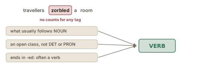
rely on the second half of the product alone, the tag that usually
follows the previous tag;
assume the unknown word belongs to an open class, since the closed
classes, determiners, pronouns and prepositions, are all already in the
corpus;
look at the shape of the word: a capital letter suggests a proper noun, a
word ending in -ly is usually an adverb, one ending in -ed a verb.
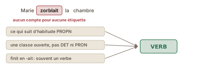
Figure 15. Three clues to the tag of a word the corpus never contained. Zorbled is an invented word.
The third strategy adds information of a new kind: not a count of the word, which does not exist, but a measurable
property of its form.
Errors that spread
The second weakness is built into the method as the worked example applies
it, from left to right. Each tag is chosen partly from the tag before it, so
a wrong tag changes the odds for the next word, and one error can produce a
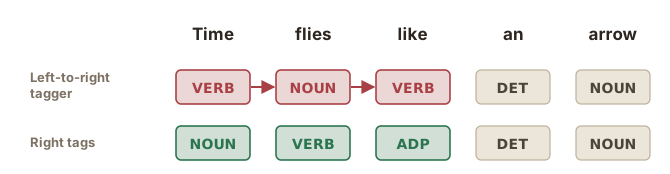
run of them. Suppose a tagger takes time in time flies like an arrow for
a verb, as in time the runners. A noun is then a likely tag for flies,
and after a noun a verb is a likely tag for like: one wrong tag has become
three (Figure 16figure 16).
A tagger that chooses the tags for the whole sentence at once can still
revise time in the light of the words after it; one that works strictly
from left to right cannot.
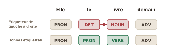
Figure 16. An illustrative left-to-right tagger that starts with one wrong tag.
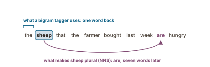
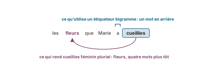
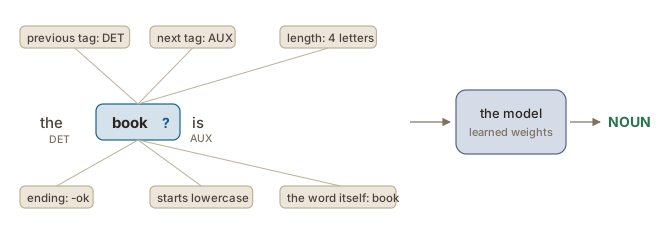
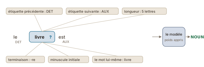
Figure 17. The context a bigram tagger uses, and the word that decides the tag.
Sources
Jurafsky, D., & Martin, J. H. (2026). Speech and Language Processing: An Introduction to Natural Language Processing, Computational Linguistics, and Speech Recognition with Language Models. Online draft, 3rd edition. https://web.stanford.edu/~jurafsky/slp3/
Manning, C. D. (2011). Part-of-speech tagging from 97% to 100%: Is it time for some linguistics?. In A. Gelbukh (Ed.), Computational Linguistics and Intelligent Text Processing, CICLing 2011 (Lecture Notes in Computer Science, Vol. 6608, pp. 171–189). Springer. https://doi.org/10.1007/978-3-642-19400-9_14
se fier à la seconde moitié du produit seule, l’étiquette qui suit
d’habitude l’étiquette précédente ;
supposer que le mot inconnu appartient à une classe ouverte, puisque les
classes fermées, déterminants, pronoms et prépositions, sont toutes déjà
dans le corpus ;
regarder la forme du mot : une majuscule suggère un nom propre, un mot en
-ment est d’habitude un adverbe, un mot en -ait un verbe.
Figure 15. Trois indices pour l'étiquette d'un mot que le corpus ne contenait pas. Zorblait est un mot inventé.
La troisième stratégie apporte une information d’un nouveau genre : non pas
un compte du mot, qui n’existe pas, mais une propriété mesurable de sa forme.
Les erreurs qui se propagent
La deuxième faiblesse tient à la méthode telle que l’exemple détaillé
l’applique, de gauche à droite. Chaque étiquette est choisie en partie
d’après l’étiquette précédente, donc une étiquette fausse change les chances
du mot suivant, et une erreur peut en entraîner une série. Supposons qu’un
étiqueteur prenne le dans elle le livre demain pour un déterminant, comme
dans le livre est long. Après un déterminant, un nom est l’étiquette la plus
probable pour livre : une étiquette fausse en a entraîné une deuxième
(Figure 16figure 16).
Un étiqueteur qui choisit les étiquettes de toute la phrase à la fois peut
encore réviser le à la lumière des mots qui suivent ; un étiqueteur qui
travaille strictement de gauche à droite ne le peut pas.
Figure 16. Un étiqueteur illustratif, de gauche à droite, qui commence par une étiquette fausse.
Figure 17. Le contexte qu'utilise un étiqueteur bigramme, et le mot qui décide de l'étiquette.
Sources
Jurafsky, D., & Martin, J. H. (2026). Speech and Language Processing: An Introduction to Natural Language Processing, Computational Linguistics, and Speech Recognition with Language Models. Online draft, 3rd edition. https://web.stanford.edu/~jurafsky/slp3/
Manning, C. D. (2011). Part-of-speech tagging from 97% to 100%: Is it time for some linguistics?. In A. Gelbukh (Ed.), Computational Linguistics and Intelligent Text Processing, CICLing 2011 (Lecture Notes in Computer Science, Vol. 6608, pp. 171–189). Springer. https://doi.org/10.1007/978-3-642-19400-9_14
Part-of-speech tagging todayL'étiquetage morphosyntaxique aujourd'hui
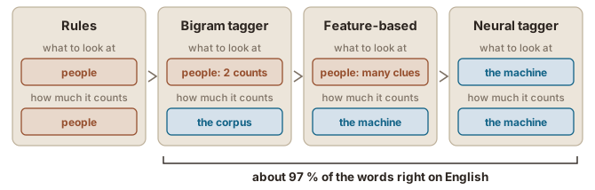
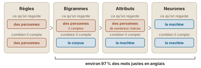
Figure 19. Four ways of tagging, from people deciding everything to the machine deciding everything. Hidden Markov model, feature-based and neural taggers all reach about 97 % on English (Jurafsky & Martin, 2026).
Where that leaves the task (Jurafsky & Martin, 2026):
What still costs: unknown words, rich morphology, and texts unlike the
training texts, such as tweets for a tagger trained on newspapers
(Manning, 2011).
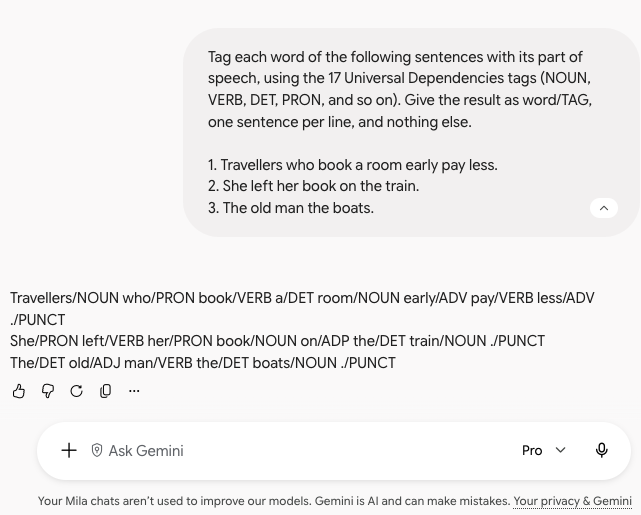
Figure 20. Gemini 3 Pro tagging three sentences with Universal Dependencies tags, captured 6 October 2026.
Where you see tagging
You will rarely run a tagger yourself, but you will see its output wherever
a tool uses grammatical classes, for instance:
the word sketches and the searches by class of a concordancer (see also the Corpus analysis module) (voir aussi le module L'analyse de corpus);
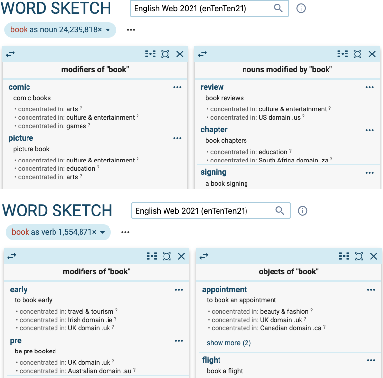
Because every occurrence in its corpus is tagged, Sketch Engine treats book
as a noun and book as a verb as two different words, with sketches that
share almost nothing
(Figure 21figure 21).
The counts show the most frequent tag at work on a real corpus: the noun is
about fifteen times as frequent as the verb.
Figure 21. Word sketches of book as a noun and as a verb in the English Web 2021 corpus (enTenTen21), Sketch Engine, captured 6 October 2026.
When such a tool makes an odd mistake, a tag wrongly assigned to an ambiguous
word is often the reason.
Sources
Jurafsky, D., & Martin, J. H. (2026). Speech and Language Processing: An Introduction to Natural Language Processing, Computational Linguistics, and Speech Recognition with Language Models. Online draft, 3rd edition. https://web.stanford.edu/~jurafsky/slp3/
Manning, C. D. (2011). Part-of-speech tagging from 97% to 100%: Is it time for some linguistics?. In A. Gelbukh (Ed.), Computational Linguistics and Intelligent Text Processing, CICLing 2011 (Lecture Notes in Computer Science, Vol. 6608, pp. 171–189). Springer. https://doi.org/10.1007/978-3-642-19400-9_14
Figure 19. Quatre façons d'étiqueter, des personnes qui décident de tout à la machine qui décide de tout. Les étiqueteurs à modèle de Markov caché, fondés sur des attributs et neuronaux atteignent tous environ 97 % en anglais (Jurafsky & Martin, 2026).
Ce qui fait encore baisser les scores : les mots inconnus, la morphologie riche, et les
textes différents des textes d’entraînement, comme des tweets pour un
étiqueteur entraîné sur des journaux (Manning, 2011).
Figure 20. Gemini 3 Pro étiquette trois phrases avec les étiquettes d'Universal Dependencies, capture du 6 octobre 2026.
Où vous voyez l’étiquetage
Vous lancerez rarement un étiqueteur vous-même, mais vous verrez ses
résultats partout où un outil se sert des classes grammaticales, par exemple :
les Word Sketches et les recherches par classe d’un
concordancier (see also the Corpus analysis module) (voir aussi le module L'analyse de corpus) ;
les vérifications grammaticales d’un traitement de texte.
Comme chaque occurrence de son corpus est étiquetée, Sketch Engine traite le
nom book et le verbe book comme deux mots différents, avec des Word Sketches qui
n’ont presque rien en commun, ici dans un corpus anglais
(Figure 21figure 21).
Les comptes montrent l’étiquette la plus fréquente à l’œuvre sur un vrai
corpus : le nom est environ quinze fois plus fréquent que le verbe.
Figure 21. Les Word Sketches de book comme nom et comme verbe dans le corpus English Web 2021 (enTenTen21), Sketch Engine, capture du 6 octobre 2026.
Quand un tel outil fait une erreur étrange, une étiquette mal attribuée à un
mot ambigu en est souvent la cause.
Sources
Jurafsky, D., & Martin, J. H. (2026). Speech and Language Processing: An Introduction to Natural Language Processing, Computational Linguistics, and Speech Recognition with Language Models. Online draft, 3rd edition. https://web.stanford.edu/~jurafsky/slp3/
Manning, C. D. (2011). Part-of-speech tagging from 97% to 100%: Is it time for some linguistics?. In A. Gelbukh (Ed.), Computational Linguistics and Intelligent Text Processing, CICLing 2011 (Lecture Notes in Computer Science, Vol. 6608, pp. 171–189). Springer. https://doi.org/10.1007/978-3-642-19400-9_14